The fastai Image classes
The fastai library is built such that the pictures loaded are wrapped in an Image. This Image contains the array of pixels associated to the picture, but also has a lot of built-in functions that will help the fastai library to process transformations applied to the corresponding image. There are also sub-classes for special types of image-like objects:
ImageSegmentfor segmentation masksImageBBoxfor bounding boxes
See the following sections for documentation of all the details of these classes. But first, let's have a quick look at the main functionality you'll need to know about.
Opening an image and converting to an Image object is easily done by using the open_image function:
img = open_image('imgs/cat_example.jpg')
img

To look at the picture that this Image contains, you can also use its show method. It will show a resized version and has more options to customize the display.
img.show()

This show method can take a few arguments (see the documentation of Image.show for details) but the two we will use the most in this documentation are:
axwhich is the matplolib.pyplot axes on which we want to show the imagetitlewhich is an optional title we can give to the image.
_,axs = plt.subplots(1,4,figsize=(12,4))
for i,ax in enumerate(axs): img.show(ax=ax, title=f'Copy {i+1}')

If you're interested in the tensor of pixels, it's stored in the data attribute of an Image.
img.data.shape
The Image classes
Image is the class that wraps every picture in the fastai library. It is subclassed to create ImageSegment and ImageBBox when dealing with segmentation and object detection tasks.
Most of the functions of the Image class deal with the internal pipeline of transforms, so they are only shown at the end of this page. The easiest way to create one is through the function open_image, as we saw before.
If div=True, pixel values are divided by 255. to become floats between 0. and 1. convert_mode is passed to PIL.Image.convert.
With the following example, you can get a feel of how open_image working with different convert_mode. For all the modes see the source here.
from fastai.vision import *
path_data = untar_data(URLs.PLANET_TINY); path_data.ls()
il = ImageList.from_folder(path_data/'train'); il
il.convert_mode = 'L'
il.open(il.items[10])

mode = '1'
open_image(il.items[10],convert_mode=mode)

As we saw, in a Jupyter Notebook, the representation of an Image is its underlying picture (shown to its full size). On top of containing the tensor of pixels of the image (and automatically doing the conversion after decoding the image), this class contains various methods for the implementation of transforms. The Image.show method also allows to pass more arguments:
This allows us to completely customize the display of an Image. We'll see examples of the y functionality below with segmentation and bounding boxes tasks, for now here is an example using the other features.
img.show(figsize=(2, 1), title='Little kitten')

img.show(figsize=(10,5), title='Big kitten')

With the following example, you will get a feel of how to set cmap for Image.show.
See matplotlib docs for cmap options here. This is how defaults.cmap is defined in fastai, see source here.
defaults = SimpleNamespace(cpus=_default_cpus, cmap='viridis', return_fig=False, silent=False)
img.shape
As cmap works on a single channel, so it is necessary to set convert_mode='L' so that the image channel will be shrinked to 1.
img = open_image('imgs/cat_example.jpg', convert_mode='L'); print(img.shape)
img

img.show(cmap='binary')

img.show(cmap='pink')

defaults.cmap = 'Blues'
img.show()

An Image object also has a few attributes that can be useful:
Image.datagives you the underlying tensor of pixelImage.shapegives you the size of that tensor (channels x height x width)Image.sizegives you the size of the image (height x width)
img.data, img.shape, img.size
For a segmentation task, the target is usually a mask. The fastai library represents it as an ImageSegment object.
To easily open a mask, the function open_mask plays the same role as open_image:
open_mask('imgs/mask_example.png')

Run length encoded masks
From time to time, you may encouter mask data as run lengh encoding string instead of picture.
df = pd.read_csv('imgs/mask_rle_sample.csv')
encoded_str = df.iloc[1]['rle_mask'];
df[:2]
You can also read a mask in run length encoding, with an extra argument shape for image size
mask = open_mask_rle(df.iloc[0]['rle_mask'], shape=(1918, 1280)).resize((1,128,128))
mask

The open_mask_rle simply make use of the helper function rle_decode
rle_decode(encoded_str, (1912, 1280)).shape
You can also convert ImageSegment to run length encoding.
type(mask)
rle_encode(mask.data)
An ImageSegment object has the same properties as an Image. The only difference is that when applying the transformations to an ImageSegment, it will ignore the functions that deal with lighting and keep values of 0 and 1. As explained earlier, it's easy to show the segmentation mask over the associated Image by using the y argument of show_image.
img = open_image('imgs/car_example.jpg')
mask = open_mask('imgs/mask_example.png')
_,axs = plt.subplots(1,3, figsize=(8,4))
img.show(ax=axs[0], title='no mask')
img.show(ax=axs[1], y=mask, title='masked')
mask.show(ax=axs[2], title='mask only', alpha=1.)

When the targets are a bunch of points, the following class will help.
Create an ImagePoints object from a flow of coordinates. Coordinates need to be scaled to the range (-1,1) which will be done in the intialization if scale is left as True. Convention is to have point coordinates in the form [y,x] unless y_first is set to False.
img = open_image('imgs/face_example.jpg')
pnts = torch.load('points.pth')
pnts = ImagePoints(FlowField(img.size, pnts))
img.show(y=pnts)

Note that the raw points are gathered in a FlowField object, which is a class that wraps together a bunch of coordinates with the corresponding image size. In fastai, we expect points to have the y coordinate first by default. The underlying data of pnts is the flow of points scaled from -1 to 1 (again with the y coordinate first):
pnts.data[:10]
For an objection detection task, the target is a bounding box containg the picture.
Create an ImageBBox object from a flow of coordinates. Those coordinates are expected to be in a FlowField with an underlying flow of size 4N, if we have N bboxes, describing for each box the top left, top right, bottom left, bottom right corners. Coordinates need to be scaled to the range (-1,1) which will be done in the intialization if scale is left as True. Convention is to have point coordinates in the form [y,x] unless y_first is set to False. labels is an optional collection of labels, which should be the same size as flow. pad_idx is used if the set of transform somehow leaves the image without any bounding boxes.
To create an ImageBBox, you can use the create helper function that takes a list of bounding boxes, the height of the input image, and the width of the input image. Each bounding box is represented by a list of four numbers: the coordinates of the corners of the box with the following convention: top, left, bottom, right.
We need to pass the dimensions of the input image so that ImageBBox can internally create the FlowField. Again, the Image.show method will display the bounding box on the same image if it's passed as a y argument.
img = open_image('imgs/car_bbox.jpg')
bbox = ImageBBox.create(*img.size, [[96, 155, 270, 351]], labels=[0], classes=['car'])
img.show(y=bbox)

To help with the conversion of images or to show them, we use these helper functions:
pil2tensor(PIL.Image.open('imgs/cat_example.jpg').convert("RGB"), np.float32).div_(255).size()
pil2tensor(PIL.Image.open('imgs/cat_example.jpg').convert("I"), np.float32).div_(255).size()
pil2tensor(PIL.Image.open('imgs/mask_example.png').convert("L"), np.float32).div_(255).size()
pil2tensor(np.random.rand(224,224,3).astype(np.float32), np.float32).size()
pil2tensor(PIL.Image.open('imgs/cat_example.jpg'), np.float32).div_(255).size()
pil2tensor(PIL.Image.open('imgs/mask_example.png'), np.float32).div_(255).size()
show_doc(tis2hw)
Visualization functions
Internally, it first creates r $\times$ c number of subplots, assigned into axes, and then loops through each of axes to create a plot with the func.
Applying transforms
All the transforms available for data augmentation in computer vision are defined in the vision.transform module. When we want to apply them to an Image, we use this method:
Before showing examples, let's take a few moments to comment those arguments a bit more:
do_resolvedecides if we resolve the random arguments by drawing new numbers or not. The intended use is to have thetfmsapplied to the inputxwithdo_resolve=True, then, if the targetyneeds to be applied data augmentation (if it's a segmentation mask or bounding box), apply thetfmstoywithdo_resolve=False.multdefault value is very important to make sure your image can pass through most recent CNNs: they divide the size of the input image by 2 multiple times so both dimensions of your picture should be mutliples of at least 32. Only change the value of this parameter if you know it will be accepted by your model.
Here are a few helper functions to help us load the examples we saw before.
def get_class_ex(): return open_image('imgs/cat_example.jpg')
def get_seg_ex(): return open_image('imgs/car_example.jpg'), open_mask('imgs/mask_example.png')
def get_pnt_ex():
    img = open_image('imgs/face_example.jpg')
    pnts = torch.load('points.pth')
    return img, ImagePoints(FlowField(img.size, pnts))
def get_bb_ex():
    img = open_image('imgs/car_bbox.jpg')
    return img, ImageBBox.create(*img.size, [[96, 155, 270, 351]], labels=[0], classes=['car'])
Now let's grab our usual bunch of transforms and see what they do.
tfms = get_transforms()
_, axs = plt.subplots(2,4,figsize=(12,6))
for ax in axs.flatten():
    img = get_class_ex().apply_tfms(tfms[0], get_class_ex(), size=224)
    img.show(ax=ax)

Now let's check what it gives for a segmentation task. Note that, as instructed by the documentation of apply_tfms, we first apply the transforms to the input, and then apply them to the target while adding do_resolve=False.
tfms = get_transforms()
_, axs = plt.subplots(2,4,figsize=(12,6))
for ax in axs.flatten():
    img,mask = get_seg_ex()
    img = img.apply_tfms(tfms[0], size=224)
    mask = mask.apply_tfms(tfms[0], do_resolve=False, size=224)
    img.show(ax=ax, y=mask)

Internally, each transforms saves the values it randomly picked into a dictionary called resolved, which it can reuse for the target.
tfms[0][4]
For points, ImagePoints will apply the transforms to the coordinates.
tfms = get_transforms()
_, axs = plt.subplots(2,4,figsize=(12,6))
for ax in axs.flatten():
    img,pnts = get_pnt_ex()
    img = img.apply_tfms(tfms[0], size=224)
    pnts = pnts.apply_tfms(tfms[0], do_resolve=False, size=224)
    img.show(ax=ax, y=pnts)

Now for the bounding box, the ImageBBox will automatically update the coordinates of the two opposite corners in its data attribute.
tfms = get_transforms()
_, axs = plt.subplots(2,4,figsize=(12,6))
for ax in axs.flatten():
    img,bbox = get_bb_ex()
    img = img.apply_tfms(tfms[0], size=224)
    bbox = bbox.apply_tfms(tfms[0], do_resolve=False, size=224)
    img.show(ax=ax, y=bbox)

Fastai internal pipeline
What does a transform do?
Typically, a data augmentation operation will randomly modify an image input. This operation can apply to pixels (when we modify the contrast or brightness for instance) or to coordinates (when we do a rotation, a zoom or a resize). The operations that apply to pixels can easily be coded in numpy/pytorch, directly on an array/tensor but the ones that modify the coordinates are a bit more tricky.
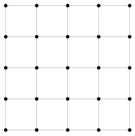
They usually come in three steps: first we create a grid of coordinates for our picture: this is an array of size h * w * 2 (h for height, w for width in the rest of this post) that contains in position i,j two floats representing the position of the pixel (i,j) in the picture. They could simply be the integers i and j, but since most transformations are centered with the center of the picture as origin, they’re usually rescaled to go from -1 to 1, (-1,-1) being the top left corner of the picture, (1,1) the bottom right corner (and (0,0) the center), and this can be seen as a regular grid of size h * w. Here is a what our grid would look like for a 5px by 5px image.
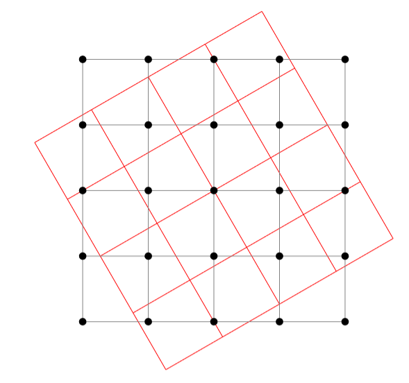
Then, we apply the transformation to modify this grid of coordinates. For instance, if we want to apply an affine transformation (like a rotation) we will transform each of those vectors x of size 2 by A @ x + b at every position in the grid. This will give us the new coordinates, as seen here in the case of our previous grid.
There are two problems that arise after the transformation: the first one is that the pixel values won’t fall exactly on the grid, and the other is that we can get values that get out of the grid (one of the coordinates is greater than 1 or lower than -1).
To solve the first problem, we use an interpolation. If we forget the rescale for a minute and go back to coordinates being integers, the result of our transformation gives us float coordinates, and we need to decide, for each (i,j), which pixel value in the original picture we need to take. The most basic interpolation called nearest neighbor would just round the floats and take the nearest integers. If we think in terms of the grid of coordinates (going from -1 to 1), the result of our transformation gives a point that isn’t in the grid, and we replace it by its nearest neighbor in the grid.
To be smarter, we can perform a bilinear interpolation. This takes an average of the values of the pixels corresponding to the four points in the grid surrounding the result of our transformation, with weights depending on how close we are to each of those points. This comes at a computational cost though, so this is where we have to be careful.
As for the values that go out of the picture, we treat them by padding it either:
- by adding zeros on the side, so the pixels that fall out will be black (zero padding)
- by replacing them by the value at the border (border padding)
- by mirroring the content of the picture on the other side (reflection padding).
Be smart and efficient
Usually, data augmentation libraries have separated the different operations. So for a resize, we’ll go through the three steps above, then if we do a random rotation, we’ll go again to do those steps, then for a zoom etc... The fastai library works differently in the sense that it will do all the transformations on the coordinates at the same time, so that we only do those three steps once, especially the last one (the interpolation) is the most heavy in computation.
The first thing is that we can regroup all affine transforms in just one pass (because an affine transform composed by an affine transform is another affine transform). This is already done in some other libraries but we pushed it one step further. We integrated the resize, the crop and any non-affine transformation of the coordinates in the same process. Let’s dig in!
- In step 1, when we create the grid, we use the new size we want for our image, so
new_h, new_w(and noth, w). This takes care of the resize operation. - In step 2, we do only one affine transformation, by multiplying all the affine matrices of the transforms we want to do beforehand (those are 3 by 3 matrices, so it’s super fast). Then we apply to the coordinates any non-affine transformation we might want (jitter, perspective wrappin, etc) before...
- Step 2.5: we crop (either center or randomly) the coordinates we want to keep. Cropping could have been done at any point, but by doing it just before the interpolation, we don’t compute pixel values that won’t be used at the end, gaining again a bit of efficiency
- Finally step 3: the final interpolation. Afterward, we can apply on the picture all the tranforms that operate pixel-wise (brightness or contrast for instance) and we’re done with data augmentation.
Note that the transforms operating on pixels are applied in two phases:
- first the transforms that deal with lighting properties are applied to the logits of the pixels. We group them together so we only need to do the conversion pixels -> logits -> pixels transformation once.
- then we apply the transforms that modify the pixel.
This is why all transforms have an attribute (such as TfmAffine, TfmCoord, TfmCrop or TfmPixel) so that the fastai library can regroup them and apply them all together at the right step. In terms of implementation:
_affine_gridis reponsible for creating the grid of coordinates_affine_multis in charge of doing the affine multiplication on that grid_grid_sampleis the function that is responsible for the interpolation step
Final result
TODO: add a comparison of speeds.
Adding a new transformation doesn't impact performance much (since the costly steps are done only once). In contrast with other libraries with classic data augmentation implementations, augmentation usually result in a longer training time.
In terms of final result, doing only one interpolation also gives a better result. If we stack several transforms and do an interpolation on each one, we approximate the true value of our coordinates in some way. This tends to blur the image a bit, which often negatively affects performance. By regrouping all the transformations together and only doing this step at the end, the image is often less blurry and the model often performs better.
See how the same rotation then zoom done separately (so there are two interpolations):
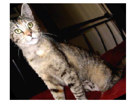
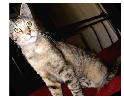
is blurrier than regrouping the transforms and doing just one interpolation:
Resize methods to transform an image to a given size:
- crop: resize so that the image fits in the desired canvas on its smaller side and crop
- pad: resize so that the image fits in the desired canvas on its bigger side and crop
- squish: resize theimage by squishing it in the desired canvas
- no: doesn't resize the image
Transform classes
The basic class that defines transformation in the fastai library is Transform.
Each argument of func in kwargs is analyzed and if it has a type annotaiton that is a random function, this function will be called to pick a value for it. This value will be stored in the resolved dictionary. Following the same idea, p is the probability for func to be called and do_run will be set to True if it was the cause, False otherwise. Setting is_random to False allows to send specific values for each parameter. use_on_y is a parameter to further control transformations for targets (e.g. Segmentation Masks). Assuming transformations on labels are turned on using tfm_y=True (in your Data Blocks pipeline), use_on_y=False can disable the transformation for labels.
func should return the 3 by 3 matrix representing the transform. The default order is 5 for such transforms.
func should take two mandatory arguments: c (the flow of coordinate) and img_size (the size of the corresponding image) and return the modified flow of coordinates. The default order is 4 for such transforms.
func takes the logits of the pixel tensor and changes them. The default order is 8 for such transforms.
func takes the pixel tensor and modifies it. The default order is 10 for such transforms.
This is a special case of TfmPixel with order set to 99.
Internal functions of the Image classes
All the Image classes have the same internal functions that deal with data augmentation.