Mixup data augmentation
What is mixup?
This module contains the implementation of a data augmentation technique called mixup. It is extremely efficient at regularizing models in computer vision (we used it to get our time to train CIFAR10 to 94% on one GPU to 6 minutes).
As the name kind of suggests, the authors of the mixup article propose training the model on mixes of the training set images. For example, suppose we’re training on CIFAR10. Instead of feeding the model the raw images, we take two images (not necessarily from the same class) and make a linear combination of them: in terms of tensors, we have:
new_image = t * image1 + (1-t) * image2
where t is a float between 0 and 1. The target we assign to that new image is the same combination of the original targets:
new_target = t * target1 + (1-t) * target2
assuming the targets are one-hot encoded (which isn’t the case in PyTorch usually). And it's as simple as that.
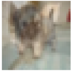
Dog or cat? The right answer here is 70% dog and 30% cat!
As the picture above shows, it’s a bit hard for the human eye to make sense of images obtained in this way (although we do see the shapes of a dog and a cat). However, it somehow makes a lot of sense to the model, which trains more efficiently. One important side note is that when training with mixup, the final loss (training or validation) will be higher than when training without it, even when the accuracy is far better: a model trained like this will make predictions that are a bit less confident.
Basic Training
To test this method, we first create a simple_cnn and train it like we did with basic_train so we can compare its results with a network trained with mixup.
path = untar_data(URLs.MNIST_SAMPLE)
data = ImageDataBunch.from_folder(path)
model = simple_cnn((3,16,16,2))
learn = Learner(data, model, metrics=[accuracy])
learn.fit(8)
Mixup implementation in the library
In the original article, the authors suggest four things:
1. Create two separate dataloaders, and draw a batch from each at every iteration to mix them up
2. Draw a value for t following a beta distribution with a parameter alpha (0.4 is suggested in their article)
3. Mix up the two batches with the same value t
4. Use one-hot encoded targets
This module's implementation is based on these suggestions, and modified where experimental results suggested changes that would improve performance.
The authors suggest using the beta distribution with parameters alpha=0.4. (In general, the beta distribution has two parameters, but in this case they're going to be equal.) Why do they suggest this? Well, with the parameters they suggest, the beta distribution looks like this:
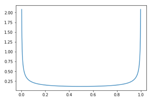
meaning that there's a very high probability of picking values close to 0 or 1 (in which case the mixed up image is mostly from only one category) and then a somewhat constant, much smaller probability of picking something in the middle (notice that 0.33 is nearly as likely as 0.5, for instance).
While this works very well, it’s not the fastest way, and this is the first suggestion we adjust. The unnecessary slowdown with this approach comes from drawing two different batches at every iteration, which means loading twice the number of images and additionally applying any other data augmentation functions to them. To avoid this, we apply mixup on a batch with a shuffled version of itself: this way, the images mixed up are still different.
Using the same value of t for the whole batch is another suggestion we modify. In our experiments, we noticed that the model trained faster if we drew a different t for every image in the batch. (Both options got to the same result in terms of accuracy, it’s just that one arrived there more slowly.)
Finally, notice that with this strategy we might create duplicate images: let’s say we are mixing image0 with image1 and image1 with image0, and that we draw t=0.1 for the first mix and t=0.9 for the second. Then
image0 * 0.1 + shuffle0 * (1-0.1) = image0 * 0.1 + image1 * 0.9
and
image1 * 0.9 + shuffle1 * (1-0.9) = image1 * 0.9 + image0 * 0.1
will be the same. Of course we have to be a bit unlucky for this to happen, but in practice, we saw a drop in accuracy when we didn't remove duplicates. To avoid this, the trick is to replace the vector of t we drew with:
t = max(t, 1-t)
The beta distribution with the two parameters equal is symmetric in any case, and this way we ensure that the largest coefficient is always near the first image (the non-shuffled batch).
Adding mixup to the mix
We now add MixUpCallback to our Learner so that it modifies our input and target accordingly. The mixup function does this for us behind the scenes, along with a few other tweaks described below:
model = simple_cnn((3,16,16,2))
learner = Learner(data, model, metrics=[accuracy]).mixup()
learner.fit(8)
Training with mixup improves the best accuracy. Note that the validation loss is higher than without mixup, because the model makes less confident predictions: without mixup, most predictions are very close to 0. or 1. (in terms of probability) whereas the model with mixup makes predictions that are more nuanced. Before using mixup, make sure you know whether it's more important to optimize lower loss or better accuracy.
Create a Callback for mixup on learn with a parameter alpha for the beta distribution. stack_x and stack_y determine whether we stack our inputs/targets with the vector lambda drawn or do the linear combination. (In general, we stack the inputs or outputs when they correspond to categories or classes and do the linear combination otherwise.)
Callback methods
You don't call these yourself - they're called by fastai's Callback system automatically to enable the class's functionality.
Draws a vector of lambda following a beta distribution with self.alpha and operates the mixup on last_input and last_target according to self.stack_x and self.stack_y.
Dealing with the loss
We often have to modify the loss so that it is compatible with mixup. PyTorch was very careful to avoid one-hot encoding targets when possible, so it seems a bit of a drag to undo this. Fortunately for us, if the loss is a classic cross-entropy, we have
loss(output, new_target) = t * loss(output, target1) + (1-t) * loss(output, target2)
so we don’t one-hot encode anything and instead just compute those two losses and find the linear combination.
The following class is used to adapt the loss for mixup. Note that the mixup function will use it to change the Learner.loss_func if necessary.