The 1cycle policy
What is 1cycle?
This Callback allows us to easily train a network using Leslie Smith's 1cycle policy. To learn more about the 1cycle technique for training neural networks check out Leslie Smith's paper and for a more graphical and intuitive explanation check out Sylvain Gugger's post.
To use our 1cycle policy we will need an optimum learning rate. We can find this learning rate by using a learning rate finder which can be called by using lr_finder. It will do a mock training by going over a large range of learning rates, then plot them against the losses. We will pick a value a bit before the minimum, where the loss still improves. Our graph would look something like this:
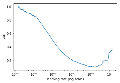
Here anything between 3x10^-2 and 10^-2 is a good idea.
Next we will apply the 1cycle policy with the chosen learning rate as the maximum learning rate. The original 1cycle policy has three steps:
1. We progressively increase our learning rate from lr_max/div_factor to lr_max and at the same time we progressively decrease our momentum from mom_max to mom_min.
2. We do the exact opposite: we progressively decrease our learning rate from lr_max to lr_max/div_factor and at the same time we progressively increase our momentum from mom_min to mom_max.
3. We further decrease our learning rate from lr_max/div_factor to lr_max/(div_factor x 100) and we keep momentum steady at mom_max.
This gives the following form:
Unpublished work has shown even better results by using only two phases: the same phase 1, followed by a second phase where we do a cosine annealing from lr_max to 0. The momentum goes from mom_min to mom_max by following the symmetric cosine (see graph a bit below).
Basic Training
The one cycle policy allows to train very quickly, a phenomenon termed superconvergence. To see this in practice, we will first train a CNN and see how our results compare when we use the OneCycleScheduler with fit_one_cycle.
path = untar_data(URLs.MNIST_SAMPLE)
data = ImageDataBunch.from_folder(path)
model = simple_cnn((3,16,16,2))
learn = Learner(data, model, metrics=[accuracy])
First lets find the optimum learning rate for our comparison by doing an LR range test.
learn.lr_find()
learn.recorder.plot()

Here 5e-2 looks like a good value, a tenth of the minimum of the curve. That's going to be the highest learning rate in 1cycle so let's try a constant training at that value.
learn.fit(2, 5e-2)
We can also see what happens when we train at a lower learning rate
model = simple_cnn((3,16,16,2))
learn = Learner(data, model, metrics=[accuracy])
learn.fit(2, 5e-3)
Training with the 1cycle policy
Now to do the same thing with 1cycle, we use fit_one_cycle.
model = simple_cnn((3,16,16,2))
learn = Learner(data, model, metrics=[accuracy])
learn.fit_one_cycle(2, 5e-2)
This gets the best of both world and we can see how we get a far better accuracy and a far lower loss in the same number of epochs. It's possible to get to the same amazing results with training at constant learning rates, that we progressively diminish, but it will take a far longer time.
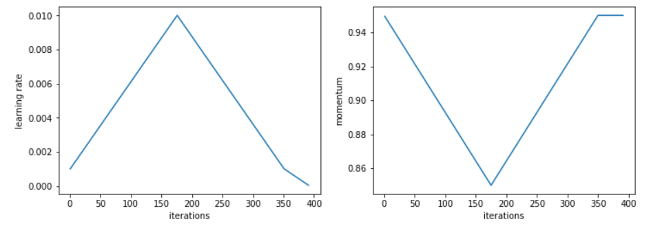
Here is the schedule of the lrs (left) and momentum (right) that the new 1cycle policy uses.
learn.recorder.plot_lr(show_moms=True)

Create a Callback that handles the hyperparameters settings following the 1cycle policy for learn. lr_max should be picked with the lr_find test. In phase 1, the learning rates goes from lr_max/div_factor to lr_max linearly while the momentum goes from moms[0] to moms[1] linearly. In phase 2, the learning rates follows a cosine annealing from lr_max to 0, as the momentum goes from moms[1] to moms[0] with the same annealing.
Callback methods
You don't call these yourself - they're called by fastai's Callback system automatically to enable the class's functionality.
Initiate the parameters of a training for n_epochs.
Prepares the hyperparameters for the next batch.